How to Find Duplicates in Excel: Complete Guide
If you're still manually searching for duplicate data in large Excel spreadsheets, this guide will show you proven methods to find duplicates in Excel in seconds. Whether you need quick visual highlighting or advanced formula-based detection, you'll find the right solution for your workflow.
Quick Method: Highlight Duplicates with Conditional Formatting
The fastest way to find duplicates in Excel is using Conditional Formatting. This built-in feature instantly highlights all duplicate values in your selected range.
Step-by-Step Instructions
- Select the data range you want to check (e.g., A2:A1000)
- Go to Home tab → Conditional Formatting
- Choose Highlight Cells Rules → Duplicate Values
- Select a highlighting color and click OK
All duplicate values will now be highlighted in your chosen color. This method works perfectly for quick visual identification.
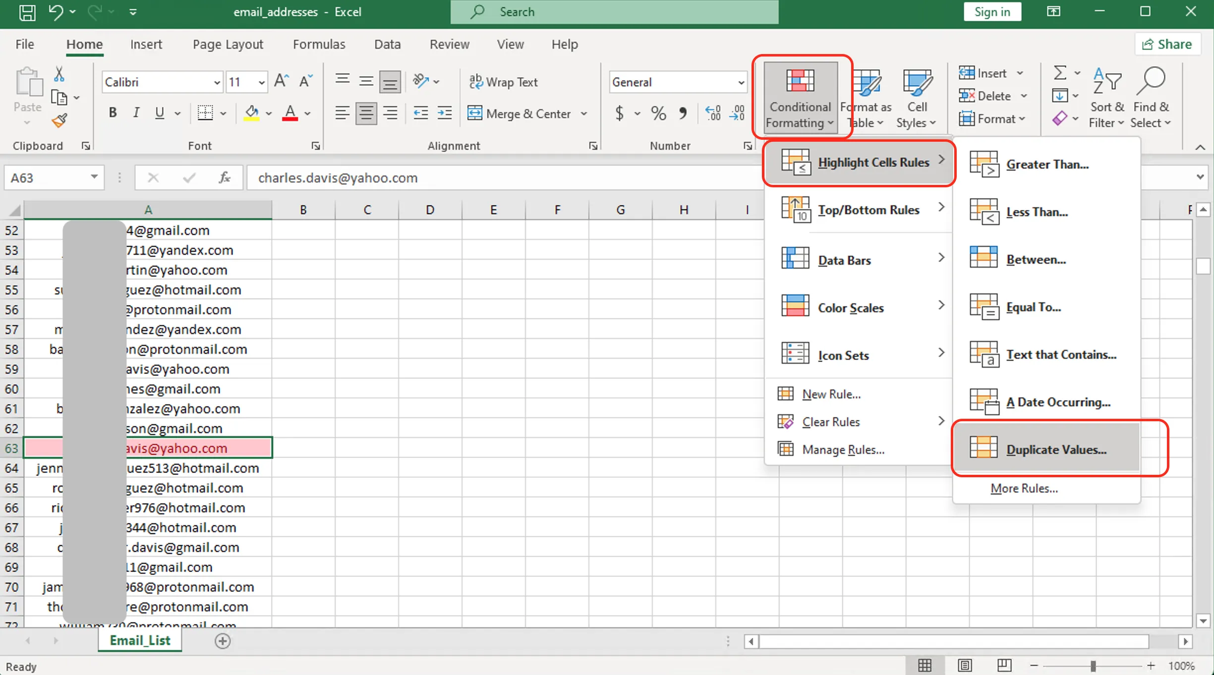
Figure 1: Excel conditional formatting duplicates highlight
=A2&B2.
Customize Duplicate Highlighting Rules
You can customize how Excel identifies duplicates:
- Duplicate: Highlights all occurrences of duplicate values
- Unique: Highlights only unique values (opposite of duplicates)
To access these options, follow the same steps above and choose 'Duplicate' or 'Unique' from the dropdown menu in the Duplicate Values dialog box.
Advanced Method: Using Formulas to Find Duplicates
For more control over duplicate detection, use Excel formulas. This approach allows you to flag duplicates in a separate column, making it easier to filter and sort.
Method 1: COUNTIF Formula
=COUNTIF($A$2:$A$1000, A2)>1This formula returns TRUE if the value in A2 appears more than once in the range.
Method 2: COUNTIF with Occurrence Number
=COUNTIF($A$2:A2, A2)This formula shows which occurrence number each entry is (1st, 2nd, 3rd, etc.). Values greater than 1 are duplicates.
Method 3: Identify First vs. Subsequent Duplicates
=IF(COUNTIF($A$2:A2, A2)>1, "Duplicate", "Original")This labels the first occurrence as 'Original' and all subsequent duplicates as 'Duplicate'.
Find Duplicates Across Multiple Columns
To find duplicates based on multiple criteria (e.g., same name AND email):
=COUNTIFS($A$2:$A$1000, A2, $B$2:$B$1000, B2)>1This formula checks if the combination of values in columns A and B appears more than once.
Remove Duplicates: Clean Your Data
After identifying duplicates, you'll likely want to remove them. Excel provides a built-in tool for this.
Steps to Remove Duplicates
- Select your data range (including headers)
- Go to Data tab → Remove Duplicates
- Choose which columns to check for duplicates
- Click OK
Excel will remove duplicate rows and show a summary of how many duplicates were removed and how many unique values remain.
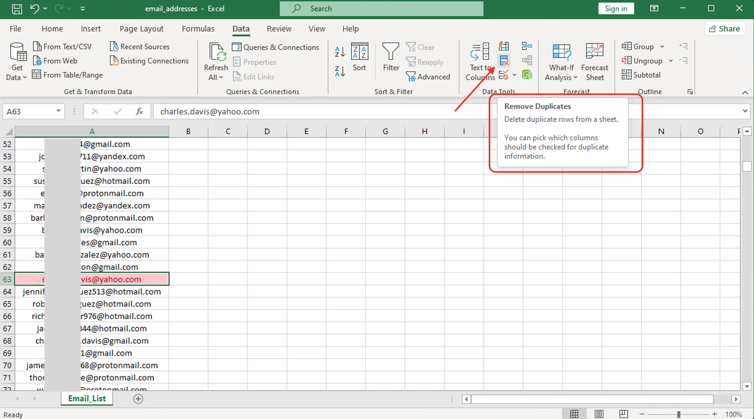
Figure 2: Excel remove duplicates tool interface
Alternative: Use the Advanced Filter to extract unique values to a new location without deleting original data.
Keep Specific Duplicates Using Sorting
If you need to keep certain duplicates (e.g., the most recent entry):
- Sort your data by the duplicate column and a timestamp column
- Use Remove Duplicates, which keeps the first occurrence
- This ensures you retain the newest or oldest entries based on your sort order
Related Resources
Ready to let Mica handle your Excel chores?
Download for Free