
If you're still losing track of column headers when scrolling through large spreadsheets, this guide will show you proven methods to freeze rows in Excel in 30 seconds. Whether you need to lock a single header row or multiple title rows, you'll find the right solution for your workflow.
Quick Answer: How to Freeze the Top Row in Excel
The fastest way to freeze a row in Excel is using the View tab:
- Click the View tab in the ribbon
- Select Freeze Panes in the Window group
- Choose Freeze Top Row from the dropdown
- A thin line appears below the frozen row
This locks your header row in place while you scroll down through thousands of rows. The frozen row stays visible at all times, eliminating confusion about which column is which.
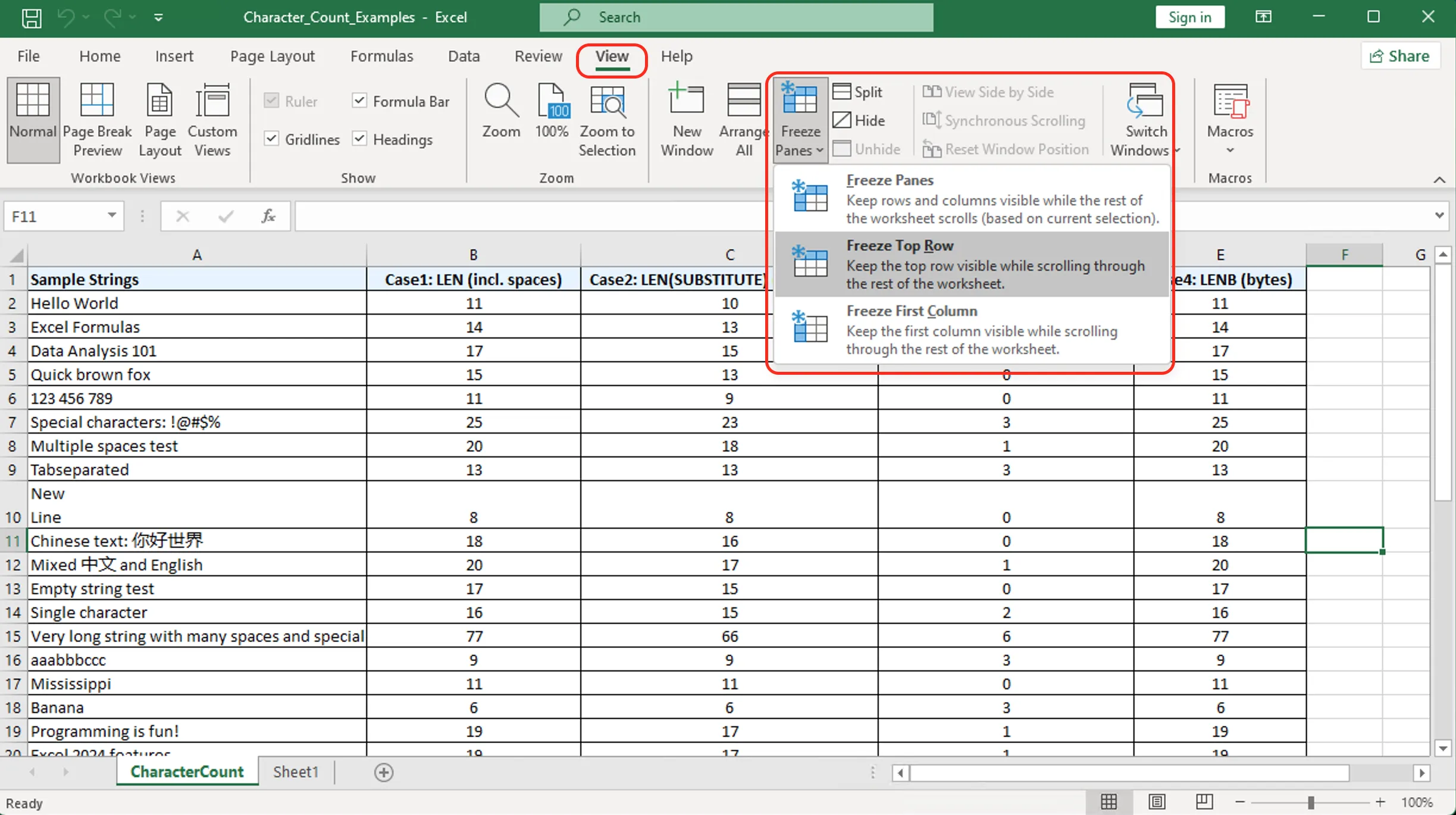
Figure 1: Freeze Top Row option in Excel's View tab
Freeze Multiple Rows: Lock Any Header Section
Need to freeze more than just the top row? Excel lets you lock multiple rows simultaneously:
Steps to Freeze Multiple Rows
- Select the row below the last row you want to freeze
- Example: To freeze rows 1-3, click row 4
- Go to View > Freeze Panes
- Click the first option: Freeze Panes
- A gray line appears above your selection
Common Scenarios
| What to Freeze | Select This Row |
|---|---|
| Row 1 only | Row 2 |
| Rows 1-2 | Row 3 |
| Rows 1-5 | Row 6 |
This is essential for complex spreadsheets with multi-level headers, company logos, or report titles that span several rows.
Freeze Panes Not Working? Common Issues Fixed
Several issues can prevent freeze panes from functioning correctly:
Issue 1: Grayed Out Freeze Panes Option
- Cause: You're in Page Layout view or Print Preview
- Fix: Go to View tab > Click Normal view
Issue 2: Frozen Row Doesn't Stay
- Cause: Workbook protection is enabled
- Fix: Review tab > Unprotect Sheet (password may be required)
Issue 3: Freeze Line Not Visible
- Cause: Thin line blends with gridlines
- Fix: The freeze is active; scroll to verify the row stays fixed
Issue 4: Want to Freeze Columns Too
- Solution: Select the cell below and to the right of what you want frozen
- Example: To freeze row 1 and column A, select cell B2
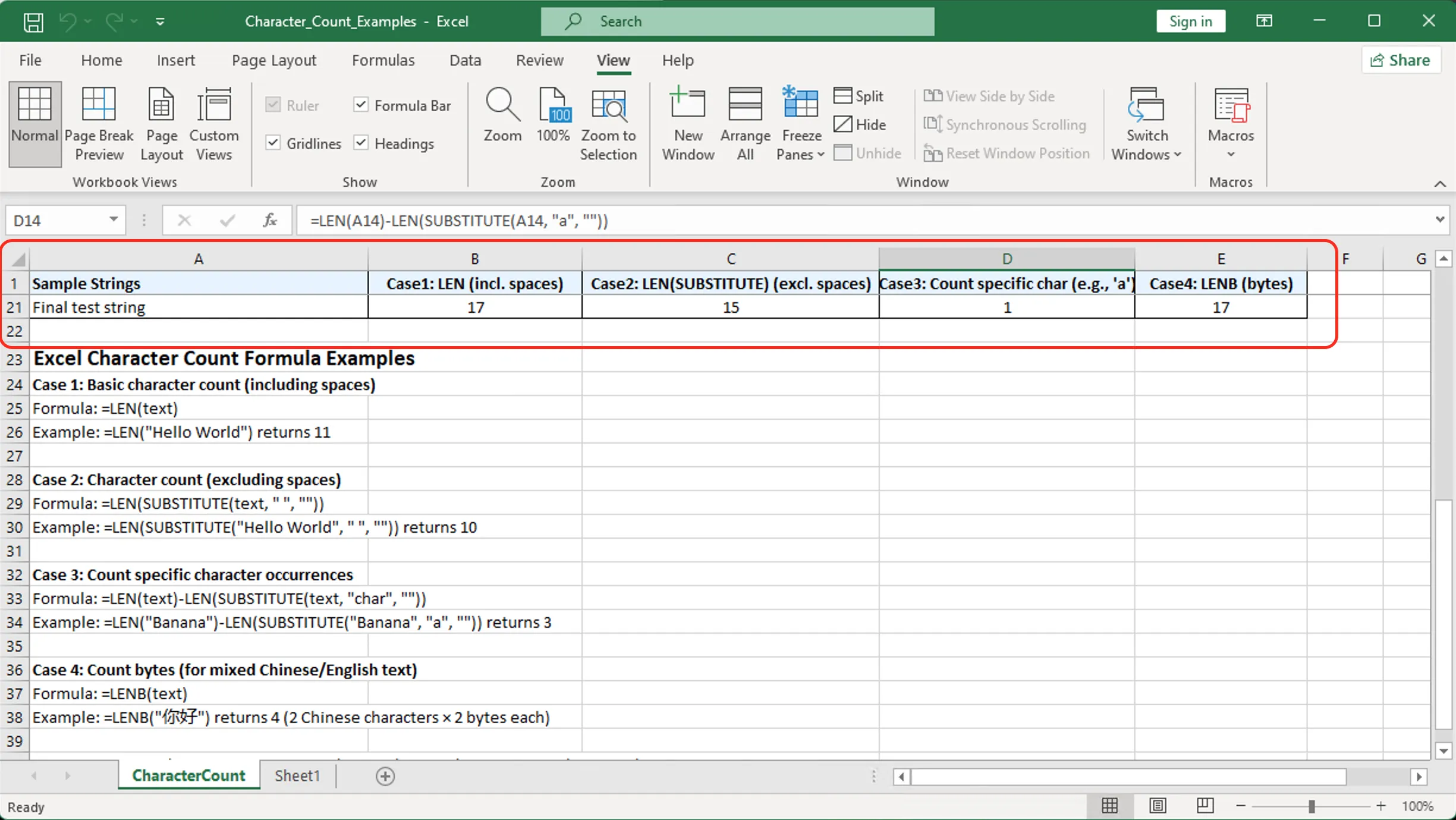
Figure 2: Before/after comparison of frozen row functionality
Keyboard Shortcuts for Freezing Rows (Windows & Mac)
Speed up your workflow with these keyboard shortcuts:
Windows
- Press
Alt+W+F+F(sequential, not simultaneous) to freeze panes - Press
Alt+W+F+Rto freeze top row only - Press
Alt+W+F+Nto unfreeze panes
Mac
- No default keyboard shortcut exists
- Workaround: Use View menu > Freeze Panes (or customize via System Preferences)
Best Practice: Always freeze headers immediately after opening large datasets before any scrolling occurs.
FAQs About Freezing Excel Rows
Can I freeze a row in the middle of my spreadsheet?
No, Excel only supports freezing from the top down. However, you can use Split view (View > Split) to create independent scrollable sections.
Does freezing rows affect printing?
No. For print headers, use Page Layout > Print Titles > Rows to repeat at top.
Will frozen rows work in Excel Online?
Yes, the Freeze Panes feature works in Excel for the Web with the same steps.
Can I freeze rows and columns simultaneously?
Yes. Select the cell below the row and right of the column you want frozen. Example: Select B2 to freeze row 1 and column A.
Why use Freeze Panes instead of Print Titles?
Freeze Panes is for on-screen viewing; Print Titles is for printed output. Use both for complete header visibility.