
The number after duration
Convexity is the curvature duration misses: 35.675 on the portfolio from the formula, 35.605 from repricing the spot curve. The finite difference has to be a second difference, because subtracting two three-price estimates amplifies round-off.
Duration gives a straight-line estimate of how a bond's price responds to yield. Convexity gives the curvature: the part the straight line misses.
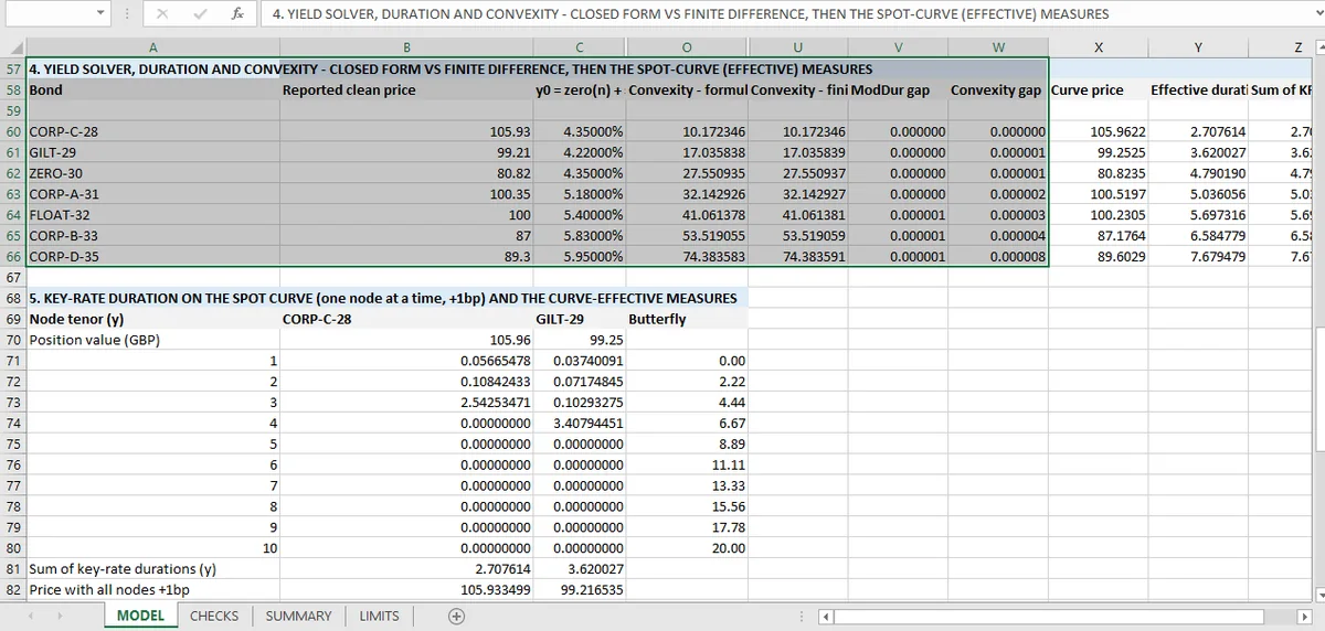
For the portfolio here, convexity is 35.675 on a flat-yield basis and 35.605 effective from the spot curve. For the first bond it is 10.172.
A larger convexity means the price rises more when yields fall than it falls when yields rise by the same amount. It is the reason a duration-only hedge is never quite flat.
Computing it from the formula
The closed form is a present-value-weighted sum of squared time, divided by price squared, with an adjustment for the compounding frequency. It is a formula in the same family as Macaulay duration, and it is easy to implement and easy to get wrong by a factor of the compounding convention.
The workbook computes it for each of the seven bonds from that formula.
Checking it by bumping
The numerical route uses a central second difference:
with h = 1 basis point, and a convention factor applied to convert the result into the quoted units.
The check is that the formula and the bump agree. They do, for all seven bonds and for the portfolio, in both the flat-yield and the spot-curve versions.
Why the bump has to be a second difference
Duration is a first derivative, so a single central difference suffices. Convexity is a second derivative, and the finite-difference version has to combine three prices rather than two.
The consequence is numerical: subtracting two numbers that are each computed from three others amplifies round-off. A bump of a tenth of a basis point would be dominated by noise; a bump of 100 basis points would truncate the curvature. One basis point is the standard compromise, and it is the one used here.
It is also why the convexity checks are the ones most likely to fail in a model that has not been tested. The analytic formula can be wrong in one direction and the numerical route in another, and the difference between them is often larger than the tolerance, which is exactly what the check is for.
What convexity buys you
The shock test in the workbook uses duration plus convexity to predict the price change under five curve scenarios, then reprices in full and compares.
The gap between the prediction and the reprice is the residue that neither first nor second order captures: third-order effects and the curve's shape. On a 1 basis point shock it is negligible; on a 100 basis point shock the prediction is visibly off, and the size of the miss is a direct measure of how much a duration-plus-convexity hedge leaves unhedged.
That is the second-order equivalent of the duration check, and it is why convexity is worth computing even when duration is the number people quote.
What neither number covers
Spread duration. The portfolio's convexity is measured against the risk-free curve; a widening of the credit spread moves the price through a different channel, and the workbook models the spread as an input rather than a dynamic quantity.
Optionality. All seven bonds are plain. A callable bond's effective convexity can be negative, and a model without an option-adjusted framework would miss it entirely. That sensitivity is the bond market's analogue of option gamma, the second derivative the derivatives workbook checks by bumping.
The shock test is where these two numbers are used together, the duration article covers the first-order piece, and the fixed income hub collects all 55. The first-order number is in the yield solve, and the exposure that survives both orders is in key-rate duration.
The analytic convexity and the bumped version are computed in adjacent cells in Mica, keeping the second-order check live. Adjacent cells are the Excel audit pattern this series uses throughout.