
A parallel shift is one scenario out of many
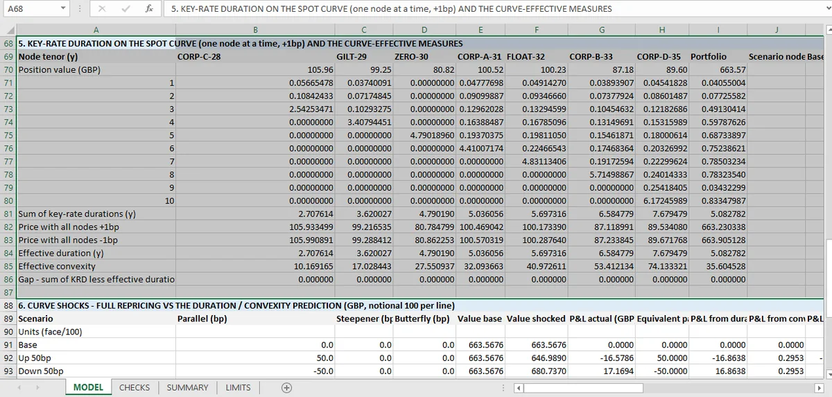
Key-rate durations decompose a 5.083-year effective duration into segments that must sum back to it. They do here, across eight checks including the portfolio. A missing segment, the 30-year point for instance, is the failure this check catches.
Effective duration answers: what happens if the whole curve moves by the same amount? Key-rate durations answer the question that follows: what if only the 5-year point moves?
The method is the same idea applied segment by segment. Bump one key rate, hold the others, reprice, measure the change. Repeat for each key rate. The result is a vector of exposures, one per segment of the curve.
For this portfolio the sum of the key-rate durations is 5.0828 years, which is exactly the effective duration under a parallel shift.
Why the sum should equal the effective duration
The additivity is not an identity by definition. It holds when two things are true.
The key rates span the curve completely. If the curve is built from 1, 2, 3, 5, 7, 10 and 30-year points and the decomposition uses only five of them, the sum falls short by the exposure in the missing segments.
The bumps are isolated and linear. Each key-rate bump changes one segment and leaves the others alone. If a bump moves a neighbouring segment through interpolation, the sum overstates the parallel effect.
When both hold, the sum of the parts equals the whole, and the workbook checks it: eight checks, seven bonds plus the portfolio, all passing.
The check is more valuable than it looks: it is the only one in the sheet that would catch a missing segment, and a missing segment is the most common key-rate error: the curve is bootstrapped to 30 years, but the risk report shows only the points with liquid instruments.
What the vector tells you that duration cannot
Two portfolios can have the same effective duration and very different key-rate profiles. One is exposed at the short end, one at the long end, and a steepening or flattening of the curve hits them in opposite directions.
That is the whole point of decomposing. A duration of 5.083 says the portfolio is exposed to parallel moves; the key-rate vector says which part of the curve matters. That decomposition is the fixed-income counterpart of risk parity contributions, which split total portfolio volatility by asset.
The workbook reports the vector and its sum, but not a comparison across portfolios, and not a steepening scenario. Those are the natural next steps and they are not present. A scenario view of the same vector is what the stress-test method adds for a multi-asset book.
What the additivity check cannot see
That the key rates are the right ones. A decomposition into 1, 5 and 10 years will sum to the effective duration if the curve is built from those three points. It will still miss the exposure between them.
That the bumps are large enough to measure. A one basis point bump on a short-dated bond produces a price change near the fourth decimal, which is where rounding lives. The workbook's tolerances allow for that; a reader taking the vector as precise should not.
That the curve is the right curve. Same limit as everywhere in this topic: the key rates are inputs.
How to read the vector
Three things worth extracting, in order.
The sum. It should equal the effective duration to within tolerance. If it does not, something is missing.
The concentration. If one segment accounts for most of the exposure, the portfolio is a bet on one part of the curve and a parallel-shift hedge will not cover it.
The sign pattern. Mixed signs mean the portfolio profits from steepening or flattening, which is a position, sometimes intended and often not.
None of that is in the workbook's summary, which reports the sum and the checks. The vector is there to be read.
The duration article covers the parallel-shift number this decomposes, the shock test is where the vector would be used against a real scenario, and all 55 checks are gathered in the fixed income hub. The flat-curve total is in the yield solve, and the curvature it leaves out is in convexity.
For the reporting side, the financial-report automation guide shows how the vector travels into a report; the Excel-for-finance guide covers the sheet mechanics.
Each key rate is bumped in its own cell in the Mica sheet, so the exposure vector and its sum recalculate together.