

Comparable Multiples: The Method That Anchors a Valuation
Comparable multiples anchor a forecast to what the market is currently paying for similar businesses.
A comparable-multiples analysis should report a distribution: quartiles, not a mean. This valuation workbook contains no peer set at all, and the article is about what one would need and how to check it.
A discounted cash flow tells you what a business is worth if your forecast is right. Comparable multiples tell you what the market is currently paying for businesses like it. Neither is an answer on its own, and a valuation with no market cross-check is a forecast wearing a valuation's clothes.
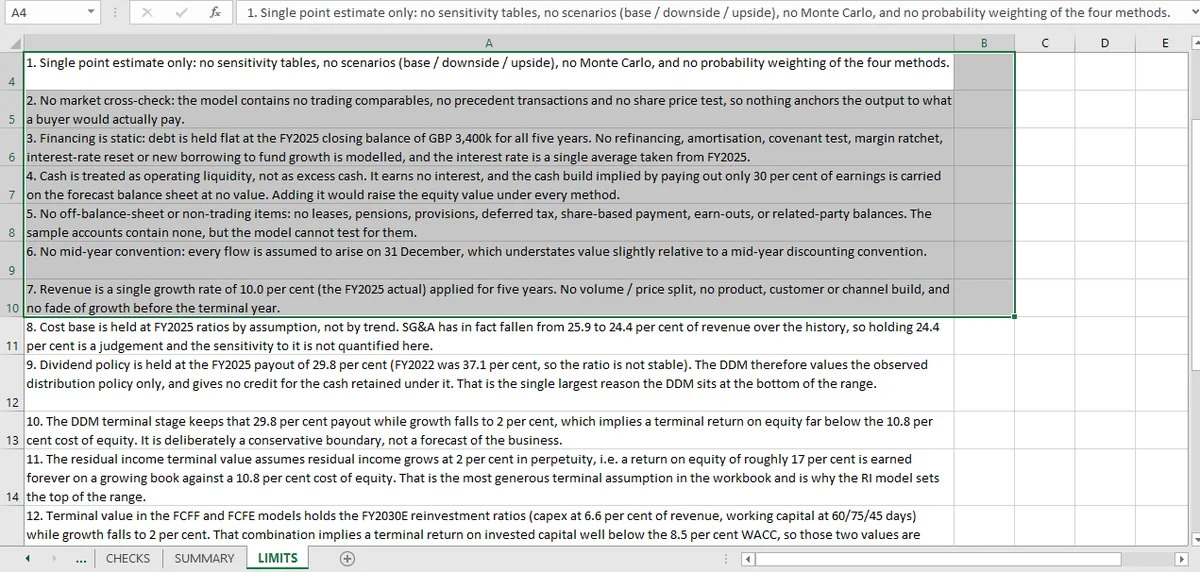
This workbook has no comps. Its limits sheet says so directly: "no trading comparables, no precedent transactions and no share price test, so nothing anchors the output to what a buyer would actually pay." That is a real gap, and this article is about what would fill it and how to check it once it exists.
A multiple is a distribution
Take twelve comparable companies, compute EV/EBITDA for each, and you have twelve numbers. Reporting the mean of them is the most common error in valuation, because the distribution of multiples is skewed and the mean sits in the tail.
The useful summary is a set of quantiles (25th, median, 75th) applied to the subject company's metric. That produces a range for the same reason the four DCF methods produce one: the inputs disagree, and the disagreement is information.
Three checks make that defensible.
The multiple is computed consistently across peers. Enterprise value means market capitalization plus net debt, using the same definition of debt for every company. A table where one peer's EV includes leases and another's does not is not a distribution; it is a random sample.
The denominator is the same period. EV/EBITDA on forward earnings and EV/EBITDA on last reported earnings are different multiples and cannot be pooled. The table should state which, in a cell, and every row should reference it.
The application is symmetric. If the range is 8.0× to 11.0×, the implied value is the subject's metric times each, and the median is the midpoint of the implied values, not the implied value of the median multiple. Those differ when the metric is negative, and they differ by construction whenever the distribution is skewed.
What comps would add to this range
The four methods here produce 7,080 to 15,439, a 74% range. That is wide enough that the range is the conclusion rather than a confidence interval around one.
A comps analysis would narrow it in a specific way: it would tell you which end of the range the market believes. If the peer set trades at 9× EBITDA and the subject's FY2030E EBITDA implies something near the top of the DCF range, the market is pricing the optimistic terminal assumption. If it implies the bottom, the market is pricing the conservative one.
The addition is not small: it converts "the value is between 7,080 and 15,439" into "the market is at 11,000, which is consistent with a terminal ROE of about 12%." The second sentence is actionable as an analytical comparison, not as a trading recommendation.
Why This Workbook Has No Comparables, and What That Costs
There are no peers because the company is synthetic, with no industry, listed comparable or transaction data.
The input pack is four years of accounts for a synthetic company. There are no peers because there is no industry, no listed comparable and no transaction data. The company does not exist.
Building a peer set from real companies and applying it to a fictional one would produce a number with no meaning, and the workbook would then be checking the arithmetic of a comparison that should not be made. Leaving it out and saying so is the right call.
What it costs the reader is the anchor. Every value in the workbook is a statement about assumptions, and none of them is a statement about what a buyer would pay. A reader who wants that has to supply the peer set themselves, and the first thing to check when they do is whether the multiples were computed consistently in the sheet. That check is worth more than a tenth of a turn of EBITDA.
How to Build a Comparable Multiples Table
Four columns are enough: EV, the metric, the multiple, and a note on the source period. Add a fifth for the definition of debt if the peer set is mixed.
Then state the applied range in three cells (low, median, high) and compute the implied equity value for each by subtracting net debt. The only arithmetic that matters is that the same metric is used in all three, and that the debt being subtracted is the same debt that was added in the enterprise value.
The rest of the valuation framework is on the valuation page; the four methods that the comps would bracket are assembled in the range article; and the next question, what happens when the multiple moves, is covered in the sensitivity piece. The DCF value a multiple would be compared against comes from the FCFF and FCFE routes.
No peer set is invented in Mica; it surfaces the inputs a model actually has, which is why the absence of comparables is visible instead of buried.