

Feasible is not optimal
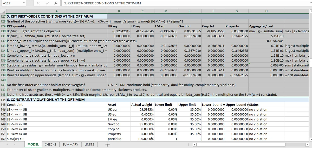
An optimum has to satisfy KKT: stationarity across free assets, complementary slackness at both bounds, dual feasibility and non-negative multipliers. The residuals here are around 10⁻¹⁰, which is solver precision rather than a tolerance somebody chose.
A constrained optimizer returns weights. The returned weights satisfy the constraints, which is the easy part. They may or may not be the best feasible point.
The difference matters. A solver that stops one iteration early returns a portfolio that sums to one, respects every cap, and leaves return on the table. Nothing in the weights themselves reveals that.
The Karush-Kuhn-Tucker conditions are the test. They are necessary conditions for a constrained optimum, and the workbook checks all of them.
The six conditions
Stationarity. At the optimum, the gradient of the objective is a combination of the constraint gradients. For a mean-variance problem, that means the marginal contribution to Sharpe is equal across every asset that is free to move. The workbook measures the largest deviation from equality: 5.2 × 10⁻¹⁰.
Complementary slackness, lower bounds. For each asset, the multiplier on the no-short constraint times the weight must be zero. If the asset is held, the multiplier is zero; if the multiplier is positive, the asset is at zero. Maximum residual: 1.5 × 10⁻¹⁰.
Complementary slackness, upper bounds. The same condition at the 35% cap. Maximum residual: 1.8 × 10⁻¹⁰.
Dual feasibility, lower and upper. The multipliers must have the right sign: non-negative for a lower bound in this formulation. Worst value: zero, exactly.
Non-negative multipliers. Every multiplier ≥ 0, checked directly.
That is six conditions, and together they cover the whole optimality claim: stationarity says you cannot improve by moving, complementary slackness says the constraints are either binding or inactive but not both, and dual feasibility says the multipliers make sense.
What Each of the Six KKT Conditions Catches
Stationarity catches a solver that stopped early. The weights can be feasible and interior while one asset still has a better marginal Sharpe than another. That is the signature of an incomplete search.
Complementary slackness catches the opposite: a solution where an asset is technically inside its bound but treated as constrained. That produces weights that overstate diversification, because the optimizer is acting as though an inactive constraint were active.
Dual feasibility catches sign errors in the solver's formulation, which usually show up as an optimum at the wrong end of a bound.
Why the residuals matter
A residual of 10⁻¹⁰ on a condition with weights of order 0.1 is not a tight tolerance. It is machine precision. The workbook is not saying "close enough"; it is saying the solver converged. The same discipline appears in the regression p-value recheck, where a reported statistic is rebuilt before it is trusted.
That is worth distinguishing from the constraint checks, which compare against 1 and 0 with a tolerance. Those are the checks a portfolio manager cares about. The KKT checks establish that the model's answer is the optimum for the stated objective and inputs; they do not say it is a portfolio anyone should hold.
The limit of the proof
KKT conditions are necessary, not sufficient, for a global optimum in a non-convex problem. Mean-variance with a positive-definite covariance matrix and linear constraints is convex, so here they are sufficient too. The workbook checks positive definiteness of the covariance matrix as part of the same group.
That check is not decoration. A covariance matrix with a negative eigenvalue makes the problem non-convex, the KKT conditions stop being sufficient, and a solver can return a local optimum that passes every stationarity test.
What is not checked
That the expected returns are right. KKT says nothing about the objective's inputs, and mean-variance is famously sensitive to them. The Black-Litterman article is where the return vector gets a prior, and the constraint article covers the feasibility side of the same solution.
All 24 checks are collected in the portfolio hub. A different objective on the same six assets is risk parity, and what the chosen weights actually earned is attribution.
The multipliers and the weights live in separate cells in the Mica sheet, so complementary slackness can be checked directly. Keeping the multiplier and the weight apart is the Excel model layout that makes the check possible.