

Three numbers from one regression
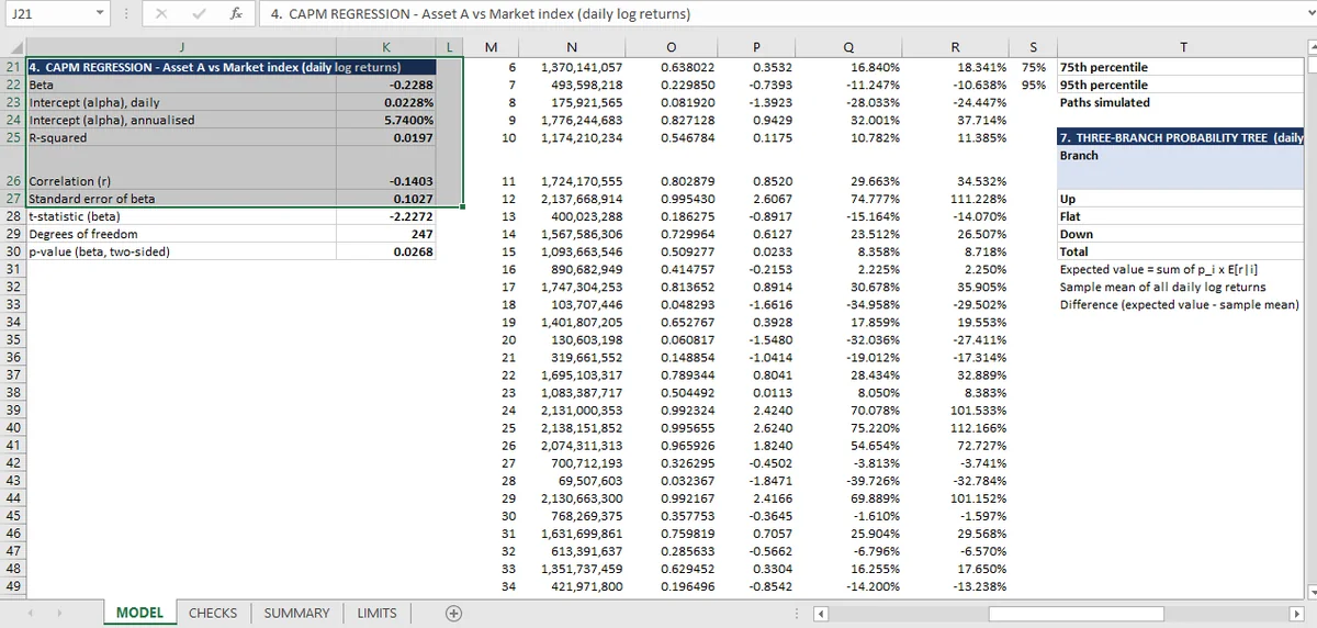
A beta of −0.229 with a p-value of 0.0268 is statistically significant at 5%. The R-squared is 0.0197, so the market explains 2% of the variation. Both numbers are reported, and together they say the relationship is real but nearly useless.
The workbook runs a regression of one asset's daily log returns on a market index and reports three numbers:
| Statistic | Value |
|---|---|
| Beta | −0.229 |
| p-value | 0.0268 |
| R-squared | 0.0197 |
Each is checked, and the checks are worth understanding because they run in different directions.
The beta identity
Beta can be computed two ways: as the slope of the regression, or as correlation times the ratio of the two volatilities.
The two paths agree here to the thirteenth decimal. That is a check on the implementation, not on the economics: it confirms the regression slope and the correlation are computed from the same series, with the same means and the same denominators.
It would fail if, say, the regression used simple returns and the correlation used log returns. The mismatch produces a beta which looks plausible and is wrong by a few percent.
R-squared is the correlation squared
The second identity: R-squared equals the correlation squared. 0.0197 for both.
This is where the three numbers start to tell a story. An R-squared of 0.0197 means the index explains 2% of the variation in the asset's returns. The other 98% is not in this regression, which makes it a data-analysis question rather than a formula one.
The p-value, and what it is a p-value for
The p-value of 0.0268 says that if the true beta were zero, a sample of 249 observations would produce a slope at least this large about 2.7% of the time. With 249 observations, that corresponds to a t-statistic of roughly 2.2.
Three things follow, and they do not all point the same way.
The sign is reliable. A p-value of 0.027 is below the conventional 5% threshold, so the negative relationship is unlikely to be an artifact of this particular sample.
The magnitude is not. A 95% confidence interval around a beta of −0.229 with t = 2.2 runs from about −0.43 to −0.03. That range includes "no useful hedge" and "a substantial short exposure".
The explanatory power is negligible. R-squared of 0.0197 is what makes the significance unsurprising: with 249 observations, almost any non-zero relationship will be significant. Significance answers "is it there"; R-squared answers "does it matter".
The check that the model runs is modest (the p-value lies in [0,1]), and it is a check against a transcription error rather than a statistical claim. A p-value of 1.7 would be a formula error; 0.0268 is plausible.
Why a check sheet cannot settle this
The checks confirm the regression is computed correctly from the series. They cannot tell you whether the regression is worth running.
That judgement depends on what the beta is for. For a hedge ratio, a beta of −0.229 with a 2% R-squared is nearly useless: the hedge would offset 2% of the variance and add its own risk. For a factor exposure in a larger model, it might be exactly the input required, with the R-squared reported alongside so that the reader knows what weight to give it. That is a modeling judgment, not an allocation recommendation.
The workbook reports both, adjacent, which is the right structure. A regression table that shows coefficients and stars but hides R-squared is the most reliable way to mislead a reader with accurate numbers.
What Would Strengthen the Regression
Three things, none of which is in the workbook.
A standard error. The p-value implies a t-statistic but the standard error is not shown, and it is the number a reader needs to construct an interval.
A second sample. Every statistic here uses all 249 observations. A split (fit on the first 150, test on the last 99) would show whether the relationship persists, which is the out-of-sample question in its simplest form.
A normality check on the residuals. The p-value assumes normal residuals. Daily returns are famously not normal, and the p-value is the number most sensitive to that assumption.
The simulation that uses the same series is the Monte Carlo article, and all 31 checks are gathered in the quantitative hub. The series both statistics come from is in returns and time value, and the simulation that assumes normal returns is in the probability tree.
The regression output sits beside the identity that checks it in the Mica sheet, so beta can be compared with correlation times the volatility ratio.