

The frontier without constraints
Constraints do not trim an efficient frontier, they move it: a 35% cap removes the maximum-return portfolio, and a no-short rule can make some risk levels unreachable. The assertions that follow are weights summing to one, no breach of either bound, and a violation count of zero.
An unconstrained mean-variance optimizer answers a simple question: for each level of risk, which mix of assets has the highest expected return? The answer is a curve. Every point on it is the mean-variance efficient portfolio at that risk, and none of them is reachable in practice.
In practice an optimizer is given bounds. No short selling. No single asset above a cap. A minimum weight in cash. Those bounds change which portfolios are admissible, and therefore which frontier is reachable.
This workbook does not contain an efficient frontier. The workbook's 31 checks cover a return series, a simulation and a regression, and the limits sheet says so. The optimizer lives in the portfolio topic, where its constraint handling is checked in a different way. This article is about what the frontier does when bounds are added, and what to assert about the result.
What a bound does to the answer
Two effects, and they are easy to confuse.
A bound can remove the maximum-return portfolio. If the highest-expected-return asset is capped at 35%, the top of the frontier is now a portfolio that holds 35% of it and 65% of other things. The frontier's endpoint moves down and right, or down and left, depending on the correlations.
A bound can make a point on the frontier unreachable. Between two constraints there may be no admissible portfolio at a given risk level. The frontier then has a gap, and the optimizer either reports the nearest reachable point or fails.
Neither effect is an error. Both mean the frontier you draw has to be the frontier of the admissible set, not of the unconstrained one. A chart that shows an unconstrained curve behind a constrained portfolio is showing two different problems.
The four assertions
Given an optimizer run with bounds, four checks cover it, and all four are cheap.
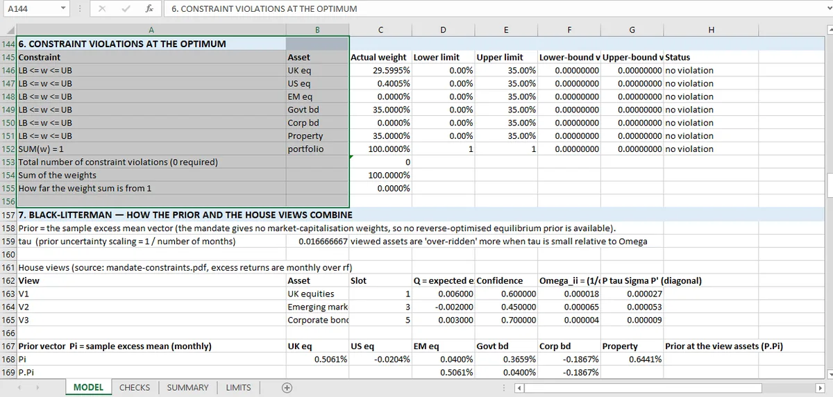
Weights sum to one. Within tolerance. A portfolio that sums to 1.0001 is 0.01% invested in nothing.
No weight below the lower bound. For a no-short constraint, the minimum is zero, and a negative weight of −0.0002 is a solver stopping one iteration early rather than a position.
No weight above the cap. The same logic at the upper end.
No constraint violated, counted. A single number, the count of violations, that must be zero. That check catches the case where a solver reports convergence while leaving one asset at 35.0001%.
The portfolio workbook runs all four and reports zero violations, with the cap exactly at 0.35 on two assets. Those two assets being exactly at the bound is itself evidence: an interior solution would not sit precisely on a constraint.
The result that looks wrong and is not
When two of six asset classes end up at zero weight and two sit exactly at the cap, the optimizer is not broken. It is telling you that the constraints are binding.
That is information. A mean-variance optimizer with a 35% cap and no shorting will concentrate wherever the risk-adjusted returns are highest, and the pattern of which assets are at zero and which are at the cap is a statement about the covariance matrix and the expected returns, not about the solver.
The failure mode to watch for is the opposite: a frontier that looks smooth and interior for every risk level. On a bounded problem that usually means the bounds are not being applied.
What constraints cost
The cost of a constraint is the return given up at the same risk, and it can be measured: optimize with and without the bound, compare the returns at a fixed volatility. The workbook does not do that, and neither does most software.
The reason is that the unconstrained optimum is often absurd: extreme weights, short positions in asset classes that cannot be shorted. That is exactly why the constraints are there. Quoting the cost of a constraint against an answer nobody could implement is not useful.
What a constrained optimum has to satisfy beyond its bounds is in the KKT article, and the constraint scan is the four-assertion version applied to a real allocation. The returns feeding any covariance matrix are in returns and time value, and the distribution behind them is in the probability tree.
Constraints become cell-level checks in the Mica build, so a violated bound appears as a failing row rather than a footnote.