

Portfolio optimization: six asset classes, one optimum
The case. Sixty months of monthly returns across six asset classes — UK equities, US equities, emerging markets, government bonds, corporate bonds and property — from a mandate and return files read as PDFs, with a 35% cap per asset and no short selling. Expected returns and the covariance matrix are inputs, not outputs; the covariance matrix is the sample matrix, with no shrinkage or factor model. One optimizer run produces the weights. This is a synthetic case for method demonstration, not investment, tax or legal advice.
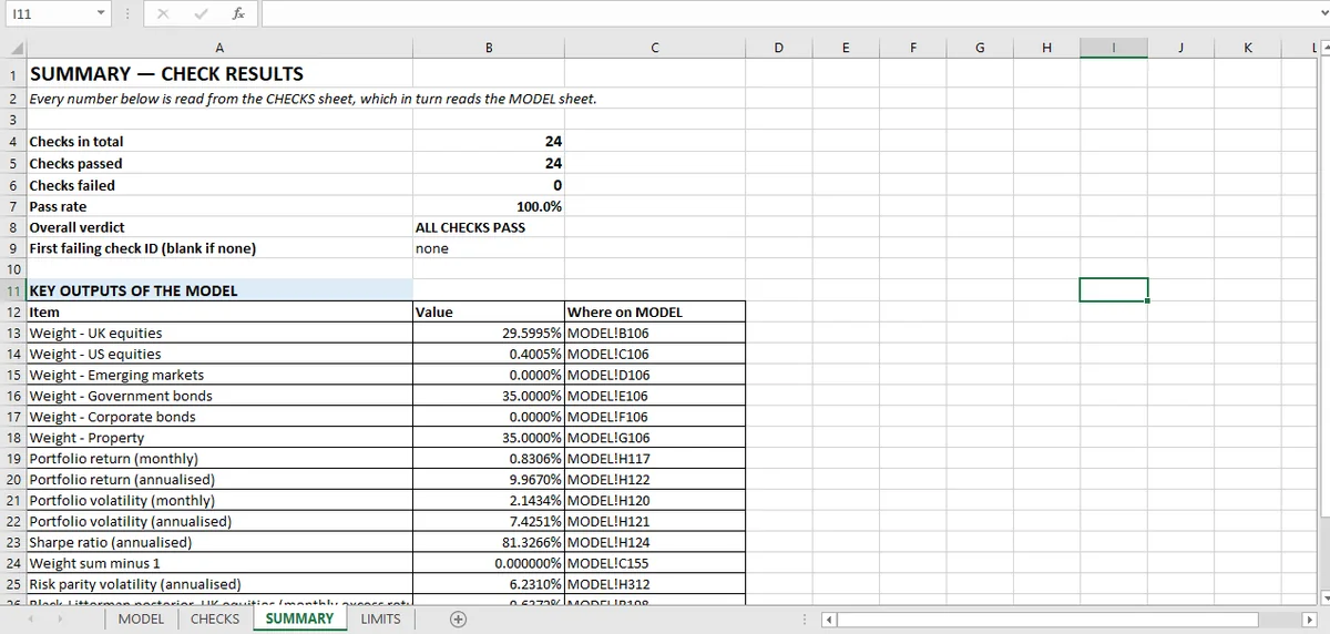
Six asset classes, a 35% cap and no shorting. The model's optimizer returns 29.6% UK equities, 0.4% US, 0% emerging markets, 35% government bonds, 0% corporate bonds and 35% property, for a Sharpe ratio of 0.813. These are the output of one run on a sample covariance matrix, not a recommended allocation.
The resulting weights:
| Asset class | Weight |
|---|---|
| UK equities | 29.6% |
| US equities | 0.4% |
| Emerging markets | 0.0% |
| Government bonds | 35.0% |
| Corporate bonds | 0.0% |
| Property | 35.0% |
| Measure | Result |
| Portfolio return, annualized | 9.97% |
| Portfolio volatility, annualized | 7.43% |
| Sharpe ratio (excess return; risk-free rate is an input) | 0.813 |
| Risk parity volatility | 6.23% |
| Weight sum minus one | 0.0000 |
The 0.813 Sharpe uses the workbook's risk-free rate as an input; the table shows the return and volatility, not the rate itself.
Twenty-four checks back the workbook. All pass.
The 24 checks prove the optimizer solved the problem it was given. The expected-return vector is the problem statement, not one of its answers.
What twenty-four checks show
Four groups, and each tests a different claim about an optimization.
Constraints (4 checks). Weights sum to one; no weight below zero; no weight above the 35% cap; zero violations at the optimum. Two assets sit exactly on the cap, which is what a binding constraint looks like.
Optimality (7 checks). The Karush-Kuhn-Tucker (KKT) conditions (stationarity, complementary slackness, dual feasibility, non-negative multipliers), plus positive definiteness of the covariance matrix and a variance-diagonal identity. Positive definiteness and the diagonal identity also appear in the input group below; the groups overlap by design, because the same property is evidence for two different claims. These are the checks that distinguish "the solver returned something feasible" from "the solver returned the optimum".
Model inputs (4 checks). The covariance matrix is positive definite; its diagonal equals the squared standard deviations; every asset has the full 60 months; the observation count matches the mandate.
Robustness and attribution (9 checks). The Black-Litterman posterior rebuilds from the prior and the views; the risk parity contributions sum to portfolio volatility and are equalised; the Brinson attribution decomposes exactly into allocation, selection and interaction.
Portfolio weights and risk parity: two results that need explaining
Two assets at zero, two at the cap. The optimizer holds no emerging markets and no corporate bonds, and holds government bonds and property at exactly 35%. That is not a solver failure; it is what a bounded mean-variance problem does. With a 35% cap and no shorting, the optimum concentrates wherever risk-adjusted return is highest, and the pattern of which assets are at a bound is information about the covariance matrix.
Risk parity produces a different volatility. The equal-risk-contribution portfolio comes out at 6.23% annualized against 7.43% for the optimized one. Different objective, different answer: mean-variance maximizes Sharpe, risk parity equalizes risk contributions regardless of expected returns. Neither is "the" portfolio, and the workbook reports both rather than picking.
The KKT checks, in plain terms
An optimizer with constraints has to satisfy Karush-Kuhn-Tucker conditions, and most software reports only the weights. This workbook checks six conditions on the solution.
The one worth understanding is complementary slackness: if an asset is inside its bound, the multiplier on that bound must be zero; if the multiplier is positive, the asset must be sitting on the bound. A solution where an interior asset carries a non-zero multiplier is not an optimum, however plausible the weights look.
The workbook's residuals on these conditions are in the 10⁻¹⁰ range, which is solver precision rather than a tolerance someone chose. The sheet layout that makes those checks possible is in the Excel-for-finance guide.
The other tests on the optimizer
The KKT conditions are how you know the solver finished. The constraint scan is four assertions that make the answer investable. Black-Litterman is where the return vector stops being a guess. Risk parity is a different objective on the same six assets. Attribution is the decomposition that has to add up. The stress test is the check the workbook does not carry. The integration article is how the 24 checks split across four different claims.
What the optimizer cannot see
Five limits, and the first is the biggest.
Expected returns are inputs. Mean-variance optimization is extremely sensitive to the return vector, and the workbook takes it as given. Nothing here tests whether the expected returns are any good. That is why the Black-Litterman section exists, and why it is a separate article.
One period, one sample. Sixty months, no regime split, no transaction costs, no turnover constraint, no rebalancing rule.
The covariance matrix is the sample one. No shrinkage, no factor model, no robustness to estimation error. The single-asset return and risk statistics that feed a covariance matrix are in the quantitative workbook.
Long-only. No leverage, no shorting, no derivatives.
No stress test. The workbook has no scenario analysis. The stress article covers what that would add and why it is the natural next check. The category-level view of why this runs as a local agent rather than a chat is in the action-bot piece.
The honest reading is that 24 checks establish the optimizer did exactly what it was asked to do with the inputs it was given. Whether those inputs produce a portfolio anyone should hold is a different question, and the workbook says so.
Bounds are applied as cell-level checks in Mica, so a binding constraint shows up in the weights and in the KKT residual at once.
Questions about the allocation
How do you check whether a portfolio optimization is correct?
Test the optimum against its own first-order conditions and constraints: weights sum to one, no weight outside its bounds, and the KKT conditions hold. This workbook runs 24 checks, including a separate constraint-violation scan, and finds zero violations.
Why does mean-variance optimization put 0% in some asset classes?
Because the optimum can sit on a constraint or an asset can add no diversification at its expected return. Here the optimizer holds 0% emerging markets and 0% corporate bonds, which is a corner solution rather than a missing input.
What Sharpe ratio is good?
There is no universal threshold; it depends on the asset classes, the period and whether returns are annualized. This portfolio achieves 0.813 at a 9.97% annualized return and 7.43% annualized volatility.
Did it respect the constraints?
Yes: weights sum to one, nothing below zero, nothing above the 35% cap, and zero violations at the optimum.