

NPV, IRR and MIRR: Three Metrics, One Question
NPV, IRR and MIRR answer the same question in three units. Here the same cash flows give 836 of NPV, a 13.15% IRR and an 11.23% MIRR. All three model outputs point to accept; the 1.92-point gap is the reinvestment assumption, not an error.
NPV, IRR and MIRR all answer the same question: does this project clear its cost of capital. They answer it in three different units.
NPV says how much value the project creates in money. IRR says what rate of return the cash flows imply. MIRR says what rate of return they imply once you state a reinvestment rate openly rather than assuming it. When the three agree, the decision is easy and the agreement tells you the cash flows are well behaved. When they disagree, the disagreement is a message about the cash flows.
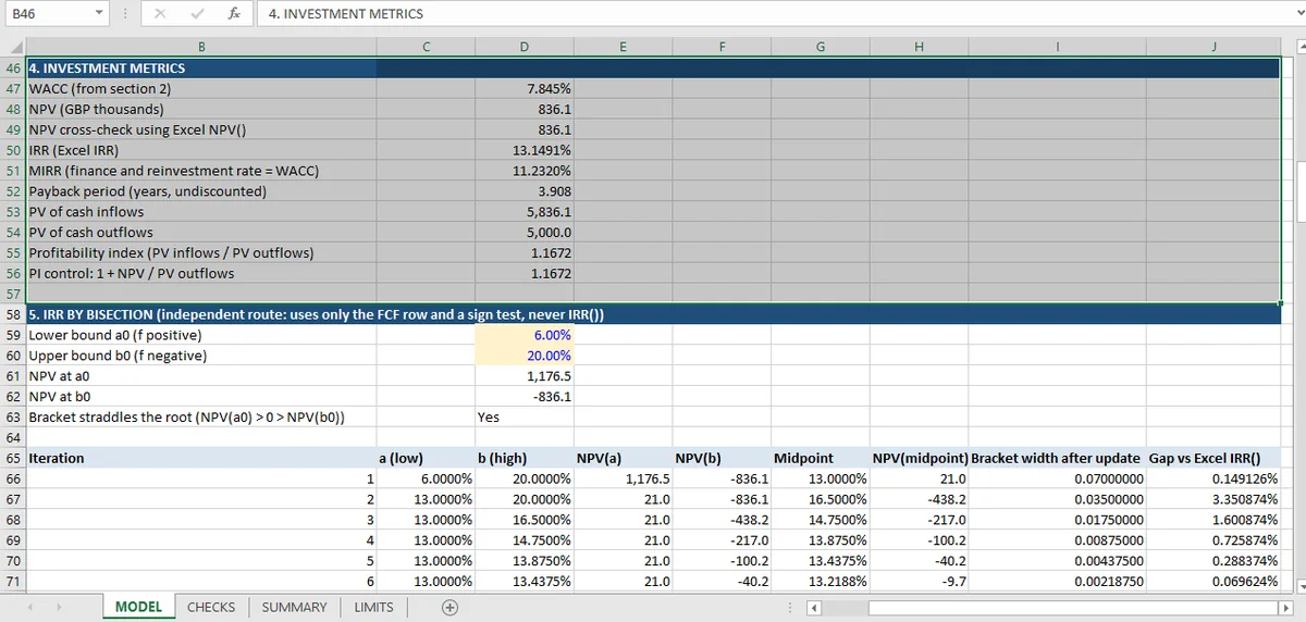
In the appraisal behind this article they agree on the decision and disagree on the number: NPV of 836 at a 7.845% WACC, an IRR of 13.15%, and an MIRR of 11.23%. All three model outputs point to accept. The 1.92-point gap between IRR and MIRR is the part worth understanding.
NPV: the number the others try to approximate
Discount the free cash flows at the cost of capital and add them up. That is the whole calculation, and it is the one metric that is not a rate: it does not depend on a reinvestment assumption, and it measures value in money rather than a ratio that can flatter a small project.
The base case runs: −5,000 at year 0, then 900, 1,312.5, 1,425, 1,500 and 2,375 across five years. At 7.845% the present values sum to 836.
Two checks confirm the arithmetic from different directions. The first recomputes the sum from the discounted cash-flow row; the second calls Excel's NPV() function on the same series. The two agree to 2 × 10⁻¹³, which is the rounding noise of double-precision arithmetic rather than a modeling difference. A third check does the thing that actually matters: it recomputes NPV at the IRR itself, and gets 8.08 × 10⁻⁸. That is below 10⁻⁷, which is what an IRR is defined to produce.
NPV is the metric to lead with because it is additive. Two projects' NPVs can be added; two IRRs cannot.
IRR: a rate that assumes reinvestment at itself
The internal rate of return is the discount rate at which NPV is zero. For this project it is 13.15%, comfortably above the 7.845% cost of capital.
The assumption buried in that number is that every interim cash flow is reinvested at 13.15% until the end of the project. That is not a forecast; it is a property of the mathematics. A firm with a 7.845% weighted average cost of capital has no reason to believe it can redeploy 1,425 from year 3 at 13.15% for the remaining two years.
In this appraisal the assumption flatters the answer slightly, because the IRR is above the WACC. For a project with early large inflows and a high IRR, the flattery can be substantial. That is one reason IRR rankings across projects of different lives are unreliable.
Excel's IRR() also has a second, quieter property: it finds one root, from a starting guess. The guess defaults to 10%, and the function returns #NUM! after 20 attempts if the iteration does not settle, as Microsoft's documentation sets out. A cash-flow series with more than one sign change can have more than one positive root, and IRR() will return whichever one its iteration happens to reach. This project's series has exactly one sign change, so there is no ambiguity here. But the model does not assume that, which is why the IRR is solved a second time.
Solving the IRR twice
The bisection block is the check worth copying into any appraisal model. It starts from a fixed bracket of 6% to 20%, and confirms the bracket straddles the root before iterating: NPV at 6% is +1,176.51, NPV at 20% is −836.05.
Then it halves the interval twenty times. The bracket narrows from 0.14 to 2.67 × 10⁻⁷, and the final midpoint is 13.149122%. Excel's IRR() returns 13.149126%. The gap is 3.4 × 10⁻⁸, or about three ten-thousandths of a basis point, and the model checks that it is under 0.0001%.
That is what a genuine convergence check looks like: two algorithms, sharing only the cash-flow row, arriving at the same number from different directions. A single method cannot tell you whether it converged or stopped.
The construction behind it — a separate block that reads only the cash-flow row, and a named rate rather than a typed one — is the pattern in the Excel-for-finance guide.
MIRR: the same cash flows with a stated reinvestment rate
MIRR removes the reinvestment assumption by stating it. Compound every inflow forward to the end of the project at a stated rate, discount every outflow back to the start at the same rate, and solve for the single rate that equates them. The Excel MIRR function names those two rates explicitly: the finance rate you pay and the reinvestment rate you receive. That is the whole point of the metric, because the assumption stops being hidden.
In this workbook both rates are set to the WACC, 7.845%, which gives 11.23%. The model does not take Excel's MIRR() on trust: a check rebuilds the future value of inflows and the present value of outflows by hand and compares.
The result is lower than the IRR by 1.92 points, and the direction is what theory predicts. Reinvesting at 7.845% rather than 13.15% reduces the return the project appears to earn, because the early cash flows no longer compound at their own rate.
Whether MIRR at the WACC is the right convention is a separate question. Using the WACC as both finance rate and reinvestment rate is a convention rather than a forecast, and the limits sheet says so. A firm that genuinely believes it can reinvest at a higher rate should say so and use that rate, with the assumption visible in a cell.
Where NPV, IRR and MIRR Diverge, and Which to Follow
All three agree here, which makes the ranking question hypothetical. The downside scenario is where it becomes concrete: revenue 10% lower gives an NPV of −277, an IRR of 6.03% and an MIRR of 6.62%.
The NPV is negative; the IRR of 6.03% and the MIRR are below the 7.845% cost of capital. All three model outputs point to reject. The ranking is unanimous because the project has a single sign change and conventional cash flows.
Where NPV and IRR genuinely conflict, it is almost always one of two cases: a project with a financing-type cash flow (an inflow first, then outflows), where IRR can invert the decision rule entirely; or two projects of different scale, where the small one can have the higher IRR and the lower NPV. In both cases NPV is the rule and IRR is the description, because NPV measures value created and the question is whether value is created.
The same conflict appears one level up, when the cash flows are a company rather than a project: the four-method valuation runs one forecast through DCF, FCFE, dividends and residual income and gets a 74%-wide range for the same reason.
MIRR sits between them: it keeps the rate format that people find easy to compare, and it removes the assumption that makes IRR misleading. It does not fix the scale problem, and it does not replace NPV.
What the checks cannot see
Six checks cover the convergence of these three metrics, and none of them can tell you whether the cash flows are right or whether the root they converge on is unique.
That second gap is worth being explicit about. Agreement between the bisection and IRR() is conditional on both converging on the same root; uniqueness requires a root count, and this workbook does not carry one. The alternative investments topic does: a fund cash flow with three sign changes and one positive root, and a comparison series with two, where IRR() quietly returns whichever root its guess reaches.
For this project the gap is theoretical: the series is −5,000 followed by five positive flows, exactly one sign change, so there is exactly one positive root by Descartes' rule of signs. The model never asserts that, though, and a reader who wants the guarantee has to check the cash-flow row themselves.
The other gap is the discount rate. An IRR of 13.15% against a 7.845% WACC is a 5.3-point margin, and how much that margin is worth depends entirely on how well the 7.845% is built.
What the checks establish is narrower than any of that: that each metric was computed from its own definition, that the definitions agree with the cash flows, and that the two algorithms for IRR converge. They do not establish that 7.845% is the right cost of capital (the WACC sensitivity article is where that number is taken apart), or that the memo's cash flows are right. For all 67 checks on this workbook, the capital budgeting hub is the place to start, or read the construction view first if you want to see how the two IRR routes are wired.
In Mica, every metric is recomputed from its own definition, which lets the reported IRR be checked against a second route in the same sheet.